Some of you know that I'm maintaining PGApack, a genetic algorithm package and a corresponding Python wrapper, PGApy. Recently the question came up why PGApack, when using Fitness Proportionate Selection (also known as Roulette-Wheel selection and also called proportional selection) errors out because it cannot normalize the fitness value.

In PGApack, the user supplies a real-valued evaluation function (which is called for each individual) and specifies if the result of that evaluation should be minimized or maximized (defining the optimization direction).

When using Fitness proportionate selection, this evaluation value must be mapped to a positive value, assigning each evaluation a share on the roulette-wheel. If the optimization direction is minimization, small values are better and need a larger part of the roulette-wheel so that they have a higher probability of being selected. So we need to remap the raw evaluation values to a nonnegative and monotonically increasing fitness. For a minimization problem, we're computing the maximum (worst) evaluation and then the fitness is the difference of this maximum and the evaluation for that individual (after scaling the maximum a little so that no fitness value is exactly zero):

where \(F\) is the fitness of the current individual, \(E_{max}\) is the maximum of all evaluations in this generation, and \(E\) is the evaluation of that individual.

Now when evaluation values differ by several orders of magnitude, it can happen that the difference in that formula ends up being \(E_{max}\) for many (different) evaluation values. I'm calling this an overflow in the error message which is probably not the best name for it.

That overflow happens when \(E_{max}\) is large compared to the current evaluation value \(E\) so that the difference ends up being \(E_{max}\) (i.e. the subtraction of \(E\) had no effect). In the code we check for this condition:

if (cmax == cmax - evalue && evalue != 0)

This condition triggers when subtracting the evaluation \(E\) from the current \(E_{max}\) does not change \(E_{max}\) even though \(E\) is not zero. So \(E\) is so small compared to \(E_{max}\) that the double data type cannot represent the difference. This happens whenever the units in the last place (called ulps by Goldberg (not the same Goldberg who wrote the Genetic Algorithms book afaik)) of the significand (also called mantissa) is larger than the value that should be subtracted [1].

In our example \(E_{max} = 1.077688 * 10^{22}\) and the evaluation where this failed was \(E = 10000\). The IEEE 754 double precision floating point format has 53 bit of significand which can represent numbers up to \(2^{54} - 1 = 18014398509481983\) or about \(1.8 * 10^{16}\). So you see that the number 10000 is just below the ulps. We can try in python (which uses double for floating-point values):

>>> 1.077688e22 - 10000 == 1.077688e22
True

Why do we make this check in the program? Letting the search continue with such an overflow (or how we want to call it) would map many different evaluation values to the same fitness. So the genetic algorithm could not distinguishing these individuals.

So what can we do about it when that error happens?

The short answer: Use a different selection scheme. There is a reason why the default in PGApack is not proportional selection.

Fitness proportionate selection (aka roulette wheel selection) has other problems, too. It has too much selection pressure in the beginning and too low at the end (also mentioned in the Wikipedia article but beware, I've written parts of it).

Blickle and Thiele [2] did a mathematical analysis of different selection schemes and showed that proportional selection is typically not a good idea (it was historically the first selection scheme and is described in Goldberg's (the other Goldberg) book [3] which is probably the reason it is still being used). Note that there is an earlier report from Blickle and Thiele [4] that is more frank about the use of proportional selection: "All the undesired properties together led us to the conclusion that proportional selection is a very unsuited selection scheme. Informally one can say that the only advantage of proportional selection is that it is so difficult to prove the disadvantages" ([4], p. 42), they were not as outspoken in the final paper :-)

We're seeing this in the example above: We have very high differences between good and bad evaluation (in fact so large that the fitness cannot be computed, see above). So when using proportional selection the very good individuals will be selected with too high probability resulting in premature convergence.

That all said: If you're doing optimization with genes of type 'real', (represented by double values in PGApack) you may want to try Differential Evolution [5], [6], [7]. At least in my experiments with antenna optimization [8] the results outperform the standard genetic algorithm, but this is reported by several practitioners [7]. Examples of how to use this are in examples/deb/optimize.c or examples/mgh/testprogde.c in PGApack.

The PGASetDECrossoverProb is critical, for problems where the dimensions cannot typically be optimized separately the value should be set close to 1 but not equal to 1.

For my pymininec project (a re-implementation of the original Mininec [1] in Python, see the pymininec README for a description on how I was able to reverse-engineer 40 year old Basic code), I had needed a method to graphically display the results. So at first I had included a visualization tool for antenna pattern in pymininec.

But after I had added a quick & dirty parser for the output of nec2c, it turned out, the program is useful on its own. So I made it a standalone program and named it plot-antenna.

NEC (numerical electromagnetics code) was originally developed at the Lawrence Livermore National Laboratory in Fortran. Up to version 2 this is free software, later versions (they're at version 5 of NEC now) are non-free. Neoklis Kyriazis translated the Fortran version of NEC-2 to C and called it nec2c. He did some optimizations, e.g. include the separate program SOMNEC (for computing a Sommerfeld/Norton ground model) directly into nec2c and got rid of many compile-time limits of the original Fortran code. The C version nec2c is one of a small number of open source antenna modelling programs. It is a command-line utility that compiles an antenna description into an output text file with a lot of tables. There are other programs like xnecview that can display antenna pattern from this output.

Note that I didn't find an official web-page for nec2c – it is included in Debian and Ubuntu (Ubuntu also is searching for the official upstream version) and it seems it was originally hosted on Google Code. There is a version on github with a link to another version on github. The software seems to be unmaintained these days – not much of a problem since NEC version 2 doesn't get any updates for some decades now.

Now back to plot-antenna: Originally the program only had a parser for output of pymininec (and of the original Mininec [1] program in Basic). I later added a parser for NEC. The current parsers are quick & dirty implementations and may not be very robust – but they do work for me.

The first version used Matplotlib for the graphic display and this is still supported. Originally I had implemented azimuth and elevation pattern and a 3d display.

Recently, after having come across plotly I added html/javascript output using the plotly library. The 3d capabilities of plotly are much better than those of Matplotlib – even with 1 degree resolution of the antenna angles (i.e. 180 * 360 3D points) the display still runs smoothly in the browser (Firefox). With the Matplotlib 3D plot, we need to use 5 degree resolution (36 * 72 3D points) otherwise rotating the display is very sluggish. You can try the plotly version yourself below (or you might want the full window antenna plot):

Not to mention zooming: This works fine in plotly (using the scroll wheel of the mouse in the graphics above) and doesn't seem to be implemented at all in Matplotlib.

In the plotly version we display the plots for all frequencies in a single plot. For the 3D view all except the currently-selected frequency are hidden. You can select the frequency for which the plot should be displayed in the legend on the right side.

The best feature in plotly is the live-display of the 3D-coordinates of the surface on mouse-over. In the current implementation this displays azimuth and elevation angles as well as the absolute and relative gains at the selected point on the antenna pattern.

On the other hand I needed several workarounds in plotly:

• There is a bug in hover when displaying coordinates

• plotly does not support menus for 3D surfaces, I had to put an additional (empty, with one white dot) graphics into the same display for showing the menu. The menu is used when an antenna pattern is computed for a set of frequencies. In that case the frequencies can be selected in the menu on the right side.

• In plotly there is no way to only show a single menu item at a time. I wanted the menu buttons to behave like radio buttons in web interfaces: Clicking on a new frequency should show only the plot for the clicked-on frequency. For 3D plots it does not make much sense to show several 3D plots in a single display. This is achieved with some custom Javascript.

The antenna pattern in the example above is taken from an article by L.B. Cebik [2]. When you compare the pattern in that article to the 3D pattern above (or you look at the azimuth/elevation diagrams in the description of plot-antenna), you'll notice that the plotly 3D view is slighty distorted (the lobe is too long). I've not yet found out if this is a problem of plotly or my use of it. I do try to get an equal aspect ratio in all dimensions by setting xaxis, yaxis, and zaxis range to the same value but as you can see the aspect ratio does not look right.

When we compare this to an azimuth diagram created with plotly:

the dimensions look ok. Notice that also in the 2D diagram you can display the angle (azimuth in this case) on mouse-over. When using Matplotlib, this is also available but the cursor does not snap to the drawn pattern. So with Matplotlib you always have to guess if the cursor is now exactly at the correct position. Also note that, again, you can select the frequency to display in the frequency legend on the right side. But this time you can display the plots for several frequencies at the same time (which does not make much sense in an opaque 3D plot).

[Update 2022-10-18: Replace epsilon with delta in description of example problem 7 in pgapack]

Many optimization problems involve constraints that valid solutions must satisfy. A constrained optimization problem is typically written as a nonlinear programming problem [1].

In this problem, there are \(n\) variables (the vector \(\vec{x}\) is of size \(n\)), \(J\) inequality constraints, \(K\) equality constraints and the variable \(x_m\) must be in the range \(|x_m^l, x_m^u|\) (often called a box constraint). The functions \(f_i\) are called the objective functions. If there is more than one objective function, the problem is said to be a multi objective optimization problem as described previously in this blog [2]. In the following I will use some terms that were introduced in that earlier blog-post without further explanation.

The objective functions are not necessarily minimized (as in the formula) but can also be maximized if the best solutions to a problem requires maximization. Note that the inequality constraints are often depicted with a \(\ge\) sign but the formula can easily be changed (e.g. by multiplying with -1) to use a \(\le\) sign.

Since it is very hard to fulfil equality constraints, especially if they involve nonlinear functions of the input variables, equality constraints are often converted to inequality constraints using an δ‑neighborhood:

Where δ is chosen according to the requirements of the problem for which a solution is sought.

One very successful method of solving constrained optimization problems is to consider a lexicographic ordering of constraints and objective function values. Candidate solutions to the optimization problem are first sorted by violated constraints (typically the sum over all violated constraints) and then by the objective function value(s) [1]. When comparing two individuals during selection in the genetic algorithm there are three cases: If both individuals violate constraints, the individual with the lower constraint violation wins. If one violates constraints and the other does not, the one not violating constraints wins. In the last case where both individuals do not violate constraints the normal comparison is used (which depends on the algorithm and if we're minimizing or maximizing). This method, originally proposed by Deb [1], is implemented in the genetic algorithm package I'm maintaining, PGAPack, and my Python wrapper PGAPy for it.

With this algorithm for handling constraints, the constraints are optimized first before the algorithm "looks" at the objective function(s) at all. It often happens that the algorithm ends up searching in a region of the input space where no good solutions exist (but no constraints are violated). Hard problems often contain equality constraints (converted to inequality constraints as indicated earlier) or other "hard" constraints. In my previous blog post [2] on antenna optimization I wrote: "the optimization algorithm has a hard time finding the director solutions at all. Only in one of a handful experiments I was able to obtain the pareto front plotted above".

In that experiment I was running 50 searches and only 5 of them did not get stuck in a local optimum. A similar thing happens for the problem (7) in Deb's paper [1] which has equality constraints. I've implemented this as example problem 7 in PGAPack. It only finds a solution near the (known) optimum when \(\delta \ge 10^{-2}\) for all equality constraints (I didn't experiment with different random seeds for the optimizer, maybe a better solution would be possible with a different random seed). In the paper [1], Deb uses \(\delta = 10^{-3}\) for the same reason.

One method for handling this problem was appealing because it is so easy to understand and implement: Takahama and Sakai were first experimenting with a method for relaxing constraints during the early stages of optization with a formulation they called an α‑constrained genetic algorithm [3]. They later simplified the formulation and called the resulting algorithm ε constrained optimization. It can be applied to different optimization algorithms, not just genetic algorithms and variants [4]. Of special interest is the application of the method to differential evolution [5], [6] but of course it can also be applied to other forms of genetic algorithms.

Note that the ε in the name of the algorithm can be used for the δ used when converting an equality constraint to inequality constraints but is not limited to this case.

During the run of the optimizer in each generation a new value for ε is computed. The comparison of individuals outlined above is modified, so that an individual is handled like it was not violating any constraints if the constraint violation is below ε. So if both individuals have constraint violations larger than ε, the one with lower violation wins. If one violation is below ε and the other above, the individual with the violation below ε wins. And finally if the constraint violations of both individuals are below ε, the normal comparison takes place.

The last case is the key to the success of this algorithm: Even though the search proceeds into a direction where the constraint violations are minimized, at the same time good solutions in terms of the objective function are found.

The algorithm begins by initializing \(\varepsilon_0\) with the constraint violation of the individuum with index \(\theta\) from the initial population sorted by constraint violation, where \(\theta\) is a parameter of the algorithm between 1 and the population size, a good value uses the individuum at about 20% of the population size which is also the default in PGAPack. In each generation \(t\), \(\varepsilon_t\) is computed by

up to generation \(T_c\). After that generation, ε is set to 0. The exponent \(cp\) is between 2 and 10. The 2010 paper [6] recommends to set \(cp = 0.3 cp + 0.7 cp_\min\) at generation \(T_\lambda = 0.95 T_c\) where \(cp_\min\) is the fixed value 3. The initial value of \(cp\) is chosen so that \(\varepsilon_\lambda=10^{-5}\) at generation \(T_\lambda\) unless it is smaller than \(cp_\min\) in which case it is set to \(cp_\min\). PGAPack implements this schedule for \(cp\) by default but allows to change \(cp\) at start and during run of the optimizer, so it's possible to easily implement a different schedule for \(cp\) – the default works quite nicely, though.

With the ε constraint method, example 7 from Deb [1] can be optimized with a precision of \(10^{-6}\) in my experiments, see the epsilon_generation parameter in the optimizer example

The antenna-optimizer with an ε‑generation of 50 (that's the \(T_c\) parameter of the algorithm) gets stuck in the local optimum only in one of 50 cases, all other cases find good results:

In that picture all the solutions that are dominated by solutions from another run are drawn in black. It can be seen that the data from run number 16 did not contribute any non-dominated solutions (on the right side in the legend the number 16 is missing). You can turn off the display of the dominated solutions by clicking on the black dot in the legend.

When I increase the ε‑generation to 60, the run with random seed 16 also finds a solution:

We also see that the solutions are quite good (quite near to the pareto front) for all runs, the black "shadow" of the dominated solutions is quite near to the real pareto front and it is enough to do a single run of the algorithm for finding a good set of solutions.

Recently in the german magazine "Funkamateur", there were two articles where the author claimed that it is possible to get a better standing wave ratio (VSWR) by using a specific lengths of 50Ω cable.

The first article was about a duo-band antenna for the 70cm and 2m ham radio bands [1]. This casually mentioned that the VSWR could be improved by using a specific length of 50Ω cable and provided a link to a software by the author to compute that length (in fact it was claimed that there are different lengths of cable that would achieve that purpose). It was claimed that this length of cable can transform the impedance (the word used was "Leitungstransformation").

In a second article – prompted by several readers who wrote letters to the editor – the author provided measurements that clearly showed that, indeed, the VSWR was improved with a certain length of cable [2].

Now transmission line theory says that a transformation resulting in a different VSWR can only be achieved by a piece of line with a different impedance that the characteristic impedance of the system, see my recent article on the subject. So there must be another reason why the impedance is changed – as clearly shown by the authors measurements. The author of the article claimed here that there is a discrepance between theory and practice – I'll show in the following that there is a reasonable explanation for the findings without dumping the existing electromagnetics theory.

The hint here is that the author did not use a balun or any other means that prevents current on the outer sheath of the feedline. So I had some fun modelling the setup with the antenna simulation program NEC2. The results should be reproduceable with any other antenna simulation program, at least if it contains a NEC core (e.g. EZNEC) which can model ground and not just free space. I've modelled the (simple two-element) antenna from the original article.

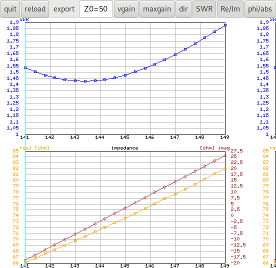
The following image shows the standing wave ratio (VSWR) and the impedance split into real and imaginary part directly at the antenna. The first NEC input file can be used to reproduce the results. Note that I'm using a Sommerfeld/Norton ground model with a medium quality ground. The antenna is located 15m above ground in the model because the antenna is meant to be used on a balcony.

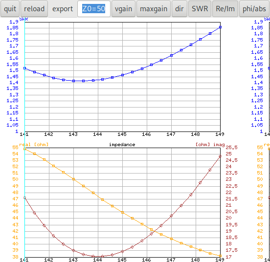
The next image shows the same antenna with a length of feedline (the length is the one for which the author claims that it can improve the VSWR). Note that the feedline is not modelled as a piece of wire but as a transmission line (which NEC provides as an abstraction). Again we show real and imaginary part. The electrical length (NEC uses only the electrical length when modeling transmission lines, no velocity factor is necessary) is about 1.81m computed by the formula in [1] with a velocity-factor of 1. It can be clearly seen that the impedance changes but the VSWR stays the same. The corresponding second NEC input file can be used to reproduce these results.

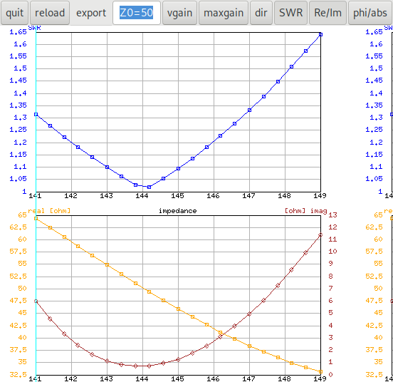
Now to simulate the conditions at the feedpoint when there is no balun I've modeled a wire between the antenna and the feedpoint at the end of the cable in the third NEC input file. The following image shows the model, we have an additional wire which represents the outside of the coax feedline. It is connected to the antenna at one point and to the end of the coax at the second point. The length of the cable is the physical length. Except for a small increase of the electrical length due to the isolation (not with the usual coax velocity factor, we're simulating only the outer braid!) the cable in the model needs to use the real physical length of the coax as computed by the formula in the first article [1]. We're using 1.484m from [1], table 3 for an Aircell5 with the factor n=1 in the table. Now we see that, indeed, as observed in the second article [2], the standing wave ratio VSWR is indeed smaller. The reason is, that due to a missing balun, the antenna itself has changed: The outer braid of the feedline is part of the antenna.

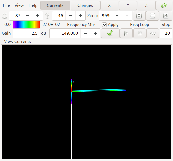
A view with the Linux program xnec2c shows the currents in the antenna and on the outer braid of the feedline. We can clearly see that there is current on the outer braid of the feedline (the feedline in the picture is the long part to the right, in parallel to that the modelled transmission line is shown).

So the electromagnetics theory is saved, there is a physical explanation of the phenomenon. It would still be interesting to model different influences like height above ground or different ground characteristics – and find out if the results above are reproduceable with different parameters since the author claims that the observed behaviour is well known ([2] p. 35).