Multi-Objective Antenna Optimization
For quite some time I'm optimizing antennas using genetic algorithms. I'm using the pgapack parallel genetic algorithm package originally by David Levine from Argonne National Laboratory which I'm maintaining. Longer than maintaining pgapack I'm developing a Python wrapper for pgapack called pgapy.
For the antenna simulation part I'm using Tim Molteno's PyNEC, a python wrapper for the Numerical Electromagnetics Code (NEC) version 2 written in C++ (aka NEC++) and wrapped for Python.
Using these packages I've written a small open source framework to optimize antennas called antenna-optimizer. This can use traditional genetic algorithm method with bit-strings as genes as well as a floating-point representation with operators suited for floating-point genes.
The parallel in pgapack tells us that the evaluation function of the genetic algorithm can be parallelized. When optimizing antennas we simulate each candidate parameters for an antenna using the antenna simulation of PyNEC. Antenna simulation is still (the original NEC code is from the 1980s and was conceived using punched cards for I/O) a CPU-intensive undertaking. So the fact that with pgapack we can run many simulations in parallel using the message passing interface (MPI) standard [1] is good news.
For pgapack – and also for pgapy – I've recently implemented some classic algorithms that have proven very useful over time:
Differential Evolution [2], [3], [4] is a very successful optimization algorithm for floating-point genes that is very interesting for electromagnetics problems
The elitist Nondominated Sorting Genetic Algorithm NSGA-II [5] allows to optimize multiple objectives in a single run of the optimizer
We can have constraints on the optimization using constraint functions that are minimized. For a solution to be valid, all constraints must be zero or negative. [6]
Traditionally with genetic algorithms only a single evaluation function, also called objective function is possible. With NSGA-II it is possible to have several objective functions. We call such an algorithm a multi-objective optimization algorithm.
For antenna simulation this means that we don't need to combine different antenna criteria like gain, forward/backward ratio, and standing wave ratio (VSWR) into a single evaluation function which I was using in antenna-optimizer, but instead we can specify them separately and leave the optimization to the genetic search.
With multiple objectives, however, typically when a solution is better in one objective, it can be worse in another objective and vice-versa. So we are searching for solutions that are strictly better than other solutions. A solution is said to dominate another solution when it is strictly better in one objective but not worse in any other objective. All solutions that fulfill this criterion are said to be pareto-optimal named after the italian scientist Vilfredo Pareto who first defined the concept of pareto optimality. All solutions that fulfill the pareto optimality criterion are said to lie on a pareto front. For two objectives the pareto front can be shown in a scatter-plot as we will see below.
Since pgapack follows a "mix and match" approach to genetic algorithms we can combine successful strategies for different parts of a genetic algorithm:
We can use Differential Evolution just for the mutation/crossover part of the genetic algorithm
We can combine this with the nondominated sorting replacement of NSGA-II
We can define some of our objectives as constraints. For our problem it makes sense to only allow antennas that do not exceed a given standing-wave ratio. So we do not allow antennas with a VSWR > 1.8. The necessary constraint function is \(S - 1.8 \le 0\) where \(S\) is the voltage standing wave ratio (VSWR).
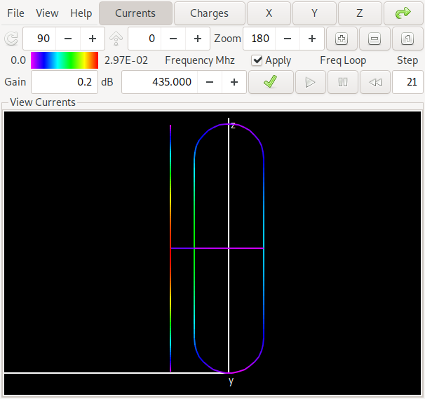
With this combination we can successfully compute antennas for the 70cm ham-radio band (430 MHz - 440 MHz). The antenna uses what we call a folded dipole (the thing with the rounded corners) and a straight element. The measures in the figure represent the lenghts optimized by the genetic algorithm. The two dots in the middle of the folded dipole element represent the point where the antenna feed-line is connected.

A first example simulates antenna parameters for the lowest, the highest and the medium frequency. The gain and forward/backward ratio are computed for the medium frequency only:
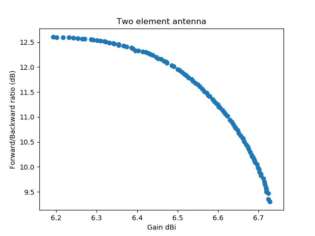
In this graph (a scatter plot) the first objective (the gain) is graphed against the second objective, the forward/backward ratio. All numbers are taken from the medium frequency. Each dot represents a simulated antenna. All antennas have a VSWR lower than 1.8 on the minimum, medium, and maximum frequency.
With this success I was experimenting with different settings of the Differential Evolution parameters. It is well-known that Differential Evolution performance on decomposable problems is better with a low crossover-rate, while it is better on non-decomposable problems with a high crossover rate. A decomposable problem is one where the different dimensions can be optimized separately, this was first observed by Salomon in 1996 [7]. I had been using a crossover-rate of 0.2 and my hope was that the optimization would be better and faster with a higher crossover rate. The experiment below uses a crossover-rate of 0.9.
In addition I was experimenting with dither: Differential Evolution allows to randomly change the scale-factor \(F\), by which the difference of two vectors is multiplied slightly for each generated variation. In the first implementation I was setting dither to 0, now I had a dither of 0.2. Imagine my surprise when with these settings I found a completely different Pareto front for the solution:
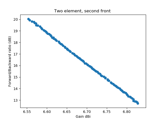
To make it easier to see that the second discovered front completely dominates the front that was first discovered, I've plotted the two fronts into a single graph:
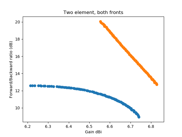
Now since the second discovered front looks too good to be true (over the whole frequency range) for a two-element antenna, lets take a look what is happening here. First we show the orientation of the antenna and the computed gain pattern for one of the antennas from the middle of the lower front:
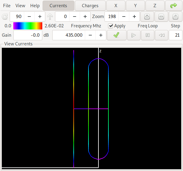
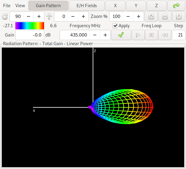
The antenna has – as already indicated in the pareto-front graphics – a gain of about 6.6 dBi and a forward/backward ratio of about 11 dB in the middle of the band at 435 MHz. The colors on the antenna denote the currents on the antenna structure. If you want to look at this yourself, here is a link to the NEC input file for antenna 1
Now lets compare this with one of the antennas of the "orange front", where we get a lot better values:
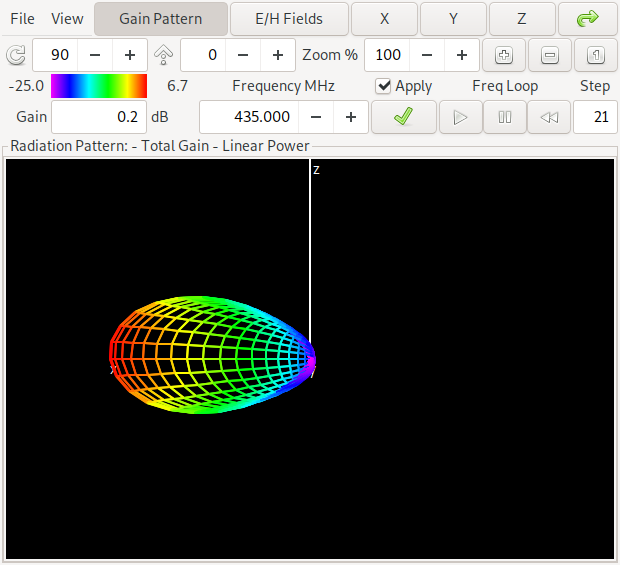
This antenna is in the middle of the pareto front above and has a gain of about 6.7 dBi and a forward/backward ratio of about 16 dB in the middle of the band at 435 MHz. Can you spot the difference to the first antenna? Yes: The maximum gain is in the opposite direction of the first antenna. We say that for the first antenna the straight element acts as a reflector while for the second antenna it acts as a director. If you want to look at this yourself, here is a link to the NEC input file for antenna 2
Now we look at the frequency plot of gain and forward/backward ratio of the antennas, the plot for the first antenna (with the reflector element) is on the left, while the plot for the antenna with the director element is on the right.
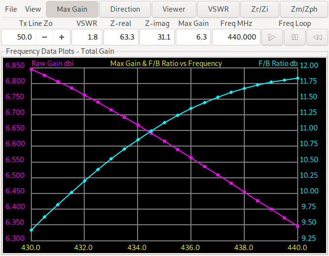
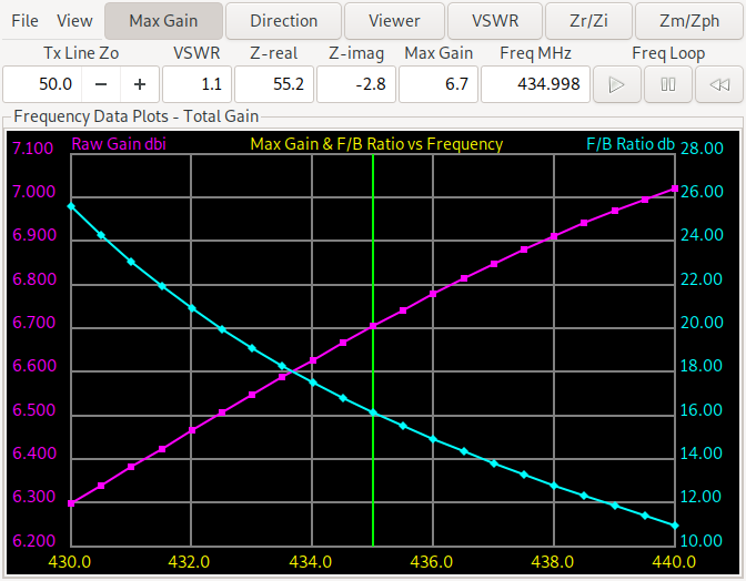
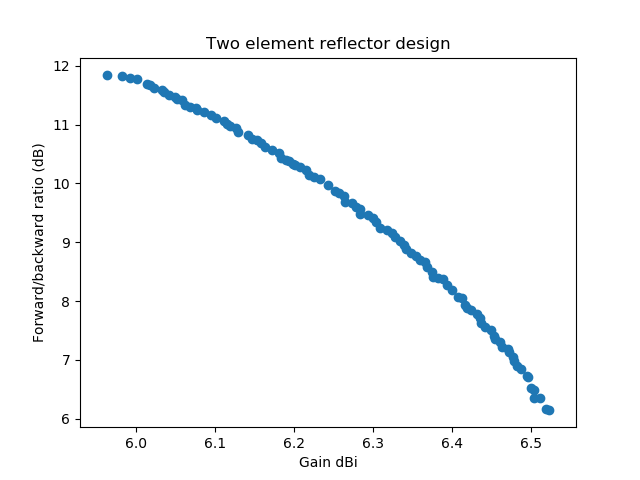
We see that the forward/backward ratio of the director antenna ranges from more than 10 dB to more than 25 dB while the reflector design ranges from 9.3 dB to 11.75 dB. For the minimum gain the reflector design is slightly better (from 6.35-6.85 dBi vs. 6.3-7.05 dBi). So this needs further experiments. When forcing a reflector design and changing the evaluation function to return the minimum gain and F/B ratio over the three (start, middle, end) frequencies we get:
The same for a director design (also with the minimum gain and F/B ratio over the three frequencies start, middle, end) we get:
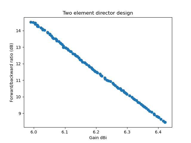
With these result, the sweet spot for an antenna to build is probably at or above 10 dB F/B ratio and a gain of about 6.2 dBi. Going for some 1/10 dBi more gain and sacrificing several dB of F/B ratio doesn't seem sensible. Comparing the director vs. reflector design we notice (contrary to at least my intuition) that the director design has a better F/B ratio over the whole frequency range. If, however the antenna is to be used for relay operation, where the sending frequency (the relay input) is in the lower half of the frequency range and the relay output (the receiving frequency) is in the upper half, we will probably chose a reflector design because there the gain is higher when sending and the F/B ratio is higher when receiving (compare the two earlier gain and F/B ratio plots).
Also note that the optimization algorithm has a hard time finding the director solutions at all. Only in one of a handful experiments I was able to obtain the pareto front plotted above. The design is more narrowband than the reflector design and the algorithm often converges to a local optimimum. The higher difference in gain and F/B range of the director design also tells us that it will be harder to build: Not getting the dimensions exactly right will probably not reach the predicted simulation results. The reflector design is a little more tolerant in this regard.