Differential Evolution Illustrated

This post again applies to PGAPack and PGApy or other Genetic Algorithm (GA) implementations that support Differential Evolution (DE).

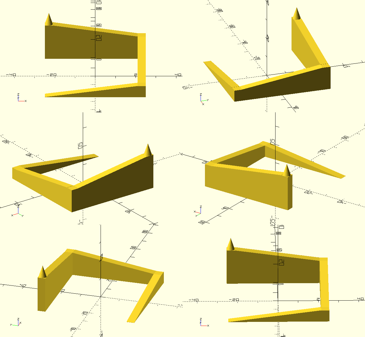
Differential Evolution (DE) [1], [2], [3] is a population based optimizer that is similar to other evolutionary algorithms. It is quite powerful and implemented in PGAPack (and usable in the Python wrapper PGAPy). To illustrate some points about this algorithm I've constructed a simple parcours in OpenSCAD.

To test the optimizer with this parcours the gene in the genetic algorithm (DE calls this the parameters) is the X and Y coordinate to give a position on the parcours. In the following we're also calling these coordinates a vector as is common in the DE literature. We initialize the population in the region of the start of the ramp. We allow the population to leave the initialization range.

Note that the corners of the parcours are flat areas with the same height. Areas like this are generally difficult for optimization algorithms because the algorithm cannot know in which direction better values (if available at all) can be found. This is also the reason why we do not put the initialization range inside the flat area at the bottom of the parcours. Note that normally one would initialize the population over the whole area to be searched. In our case we want to demonstrate that the algorithm is well capable of finding a solution far from the initialization range.

The algorithm of DE is quite simple (see, e.g. [3] p.37-47): Each member \(\mathbf x_{i,g}\) in the population of the current generation \(g\), where \(i\) is the index of the population member is crossed over with a mutant vector \(v_{i,g}\). The mutant vector is generated by selecting three population members at random (without replacement) from the population and combining them as follows.

As can be seen, the weighted difference of two random members of the population is added to a third population member. All indeces \(r_0, r_1,\) and \(r_2\) are different and different from \(i\). The weight \(F\) is a configuration parameter that is typically \(0.3 \le F < 1\). This algorithm is the classic DE, also often termed de-rand-1-bin. A variant uses the index of the best individual instead of \(r_0\) and is called de-best-1-bin. If more than a single difference is added, another variant would be, e.g., de-rand-2-bin. The last component of the name bin refers to uniform crossover [4], a binomial distribution. In DE, parameters from the mutant vector are selected with a certain probability \(Cr\). Note that DE makes sure that at least one parameter from the mutant vector is selected (otherwise the original vector \(\mathbf x_{i,g}\) would be unchanged).

More details about DE and the usage with PGAPack can be found in the section Differential Evolution and in the Mutation sections of the PGAPack documentation.

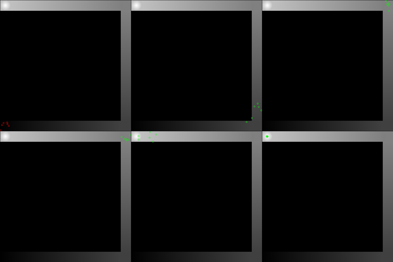
To use the OpenSCAD model for optimization, we convert it to a greyscale heightmap using an STL to PNG converter (STL is a 3D format that can be generated by OpenSCAD). The evaluation function then simply returns the greyscale value at the given location (after rounding the gene X and Y values to an integer). Values outside the picture are returned as 0 (black). The resulting optimization run is shown below in an animated image. The population is quite small, there are only 6 individuals in the population. We clearly see that when the differences between individuals gets large (on the straight ridges of the parcours), the optimization proceeds in larger steps. We also see that the flat corners can take quite some time to escape from and in the corners the algorithm slows down. Finally in the last corner, the cone is climbed and the individuals converge almost to a single point. The algorithm is stopped when the first individual returns an evaluation of the largest greyscale value (representing white). Note that I cheated a little in that many optimization runs take longer (in particular the optimization can get stuck for many generations in the flat parts of the ridge) and I selected a run that produced a good animation. So the selected run is not the average but one of the shorter runs.