Q-Factor of a Coax Resonator
When studying transmission line theory recently for modelling transmission lines in my antenna-optimizer project, I stumbled upon a formula of the Quality (Q) factor of a coax resonator by Frank Witt [1]:
In this formula \(F_0\) is the frequency of the resonator in MHz, \(A\) is the loss in dB per 100 ft, and VF is the velocity factor of the cable. The formula is for a \(\frac{\lambda}{4}\) resonator. I wondered about this because, since the loss in that formula is a logarithmic quantity (dB) the computation of the Q-factor should involve exponentiation.
When using the stored energy definition of the Q-factor from Wikipedia, we get:
where \(E_s\) is the stored energy and \(E_d\) is the energy dissipated per cycle.
We know that the loss factor of a cable in dB involves power loss. If the loss in dB per 100m (we're using metric units) is \(a\) we have for the loss in dB:
where \(l\) is the length im meter. For a \(\frac{\lambda}{4}\) resonator we get:
To compute the fraction of the power lost (instead of the logarithm of the fraction in dB) when transmitting we get
Replacing
into the formula where \(c\) is the speed of light and \(f_0\) is the resonance frequency in Hz we get
Going back to the Wikipedia formula which involves energies to get an energy ratio from a power ratio we would have to integrate – but since this would yield the same result for the ratio we instead do a handwaving integration here: We need to get the travelled distance straight: The Wikipedia definition involves one whole period \(\lambda\), not \(\frac{\lambda}{4}\). And the Q-factor is the ration of the stored power to the lost power. So we have:
Note that this makes the resonator \(Q\) independent of the type of resonator, be it a \(\frac{\lambda}{4}\) or \(\frac{\lambda}{2}\) resonator.
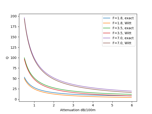
When plotting Q-factors for some shortwave frequencies (they're in MHz in the figure) against the loss in dB we see that the formula derived above is fairly close to the approximation formula from Witt [1].
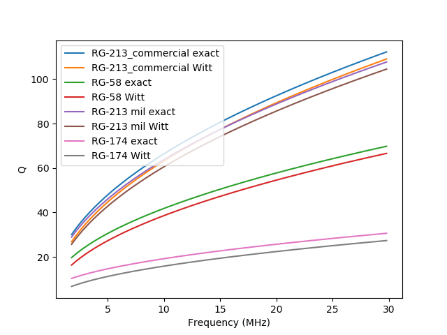
When plotting Q-factor against frequency (also in the shortwave range) for certain common cable types we also see that the error is not too high, especially for higher frequencies.
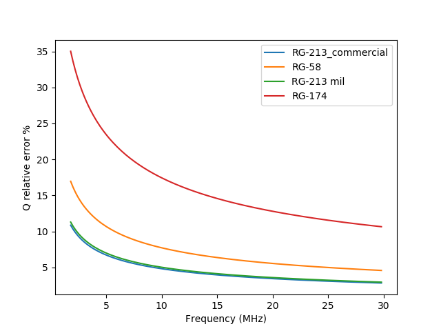
The relative errors can also be plotted, also for some common cable types over the whole shortwave range. We see that the error is quite high for the low frequency range and is higher for the more lossy cable types like RG174.
So we see that the formula is probably some approximation and is fairly accurate for higher frequencies and low loss. Now the question was open: Where does this formula come from and what is the magic constant that obviously lumps all physical constants into a magic number?
When studying transmission line theory I also stumbled over an old book on the subject which once was a university textbook [2]. On p. 222 Chipman derives an approximate formula for \(Q\) with a simplifying assumption that \(\alpha\) (the attenuation coefficient in nepers per meter) is small. Chipman's approximate formula is:
where \(\alpha\) is the attenuation coefficient in nepers per meter and \(\beta\) is the phase factor of the line in radians per meter. The subscript \(r\) stands for resonance. We can write
and
and Witts loss \(A\) per 100ft can be written (converting nepers to dB) as
Where the constant 3.2808 is the conversion factor m/ft. Solving for \(\alpha_r\) and replacing \(\lambda\) and \(\alpha_r\) into Chipman's formula we get:
Where the final \(F_0\) is \(f_0\) in MHz.
We see that the low-\(\alpha\) asumption of Chipman's (and Witt's) formula holds for higher frequencies and low loss. We've already seen that the approximation if fairly good for low-loss cables: \(\alpha\) in nepers per meter is a constant factor from the loss-figure in dB (be it per 100m or per 100ft). That it gets better with higher frequencies is because the loss of a cable typically increases with the square-root of the frequency while \(\lambda\) decreases inverse proportionally with frequency. So, e.g., a \(\frac{\lambda}{4}\) resonator has higher loss at a lower frequency.